Chapter 7: Goal Misgeneralization

Learning Dynamics

Learning Dynamics, Markov Grey

The training process guides which algorithms and goals are discovered. The results of AI training are shaped by poorly understood preferences in the training system, and what's easiest to compute.

A deeper understanding of goal misgeneralization requires examining how the training process in machine learning actually works. When we train neural networks, we're adjusting millions or billions of parameters. But what do these parameters represent? The best way to think about machine learning is as a search process through a vast space of possible algorithms (also sometimes called search through the hypothesis space or model space). Each specific combination of parameter values corresponds to a different algorithm for processing information and making decisions. The path this search takes—and the biases that guide it—determine what types of algorithms get discovered and whether they pursue intended goals or merely correlated proxies. The intuitions that you learn in this section will help you immensely both in this chapter, but also in the later chapters on interpretability.

Each point in parameter space encodes a complete algorithm. Just as the binary digits 0 and 1 can encode any computer program, the millions of floating-point parameters in a neural network encode an algorithm for solving tasks. Change some parameters, and you get a different algorithm. The network's weights determine exactly how it processes inputs—what patterns it recognizes, what features it prioritizes, what decisions it makes. Two networks with different parameter values implement different algorithms, even if they achieve similar performance.

Training often discovers algorithms that work for unexpected reasons. In the image below, if you show a human these red curved objects and say they were all "thneebs," most people would assume the defining feature is the shape. But if we use neural networks on similar examples, the networks would consistently learn that "thneeb" only means any "red object"—focusing on color rather than shape. Which is to say that if we gave them a blue object but with the same shape, then they don't consider it a “thneeb”. Both approaches achieve perfect performance during training, yet they represent completely different algorithms that would behave very differently when encountering new examples (Cotra, 2021).

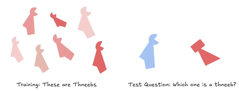
Figure 7.9: This is called a Thneeb. It is a word defined only for the sake of the experiment. The image on the left is the training data, the image on the right is the test data. If after looking at the image on the left, we ask you which one of the two on the right is a thneeb? You would probably say the left object because you generalized through the shape path, but neural networks would answer that the shape on the right is a thneeb, showing they “prefer“ the color path (Cotra, 2021; Geirhos et al., 2019).

Many algorithms can be behaviorally indistinguishable during training while pursuing completely different goals. We already made this point in the previous section but it is worth highlighting again. As another concrete example, researchers trained 100 identical BERT models on the same dataset with identical hyperparameters; all models achieved nearly indistinguishable performance during training. Yet when tested on novel sentence structures, these models revealed completely different approaches—some had learned more robust syntactic reasoning while others relied on superficial pattern matching. The training process had found 100 different algorithms in the space of possible language processing strategies (McCoy et al., 2019).

The reason we make this point again is to motivate the fact that understanding the search process—how training navigates the space of possible algorithms and which solutions it tends to discover. This is very useful for what types of AIs (parameter configurations = algorithms) we might actually end up discovering, and whether we can change something about our architectures or learning dynamics to influence this process.

Loss Landscapes

Video: The Misconception that Almost Stopped AI [How Models Learn Part 1], Welch Labs

This is the loss landscape of Meta's Llama 3.2 large language model. Virtually all modern AI models learn by gradient descent. Visually, this looks like starting at a random location on our landscape and working our way downhill towards lower loss, higher performance solutions. But how does our model avoid getting stuck in local valleys like this one? This question stopped many early AI pioneers in their tracks. Geoff Hinton, who would go on to win the Nobel Prize in 2024 for his work in AI, initially entirely dismissed training neural networks like Llama with gradient descent for exactly this reason. Of course, as we now know, gradient descent actually works unbelievably well. What understanding was Hinton missing? And what's wrong with our picture? In this series, we'll take a fresh look at how AI models learn. Starting with a visual first approach, we'll dig into how exactly our Llama model learns from real training examples, what our loss landscape can and can't show us, and ultimately see why gradient descent for large models looks more like falling into a wormhole than it does simply heading downhill. In part two, we'll switch to a more math-driven approach, which will help us grapple with the incredibly high-dimensional spaces these models operate in. Researching this series, I found some really interesting visualization techniques that required some deep focus time to get my head around, which this video's sponsor, Incogni, has really helped me with. I've been an Incogni customer for six months now and continue to be blown away by how many fewer spam texts, calls, and emails I get, giving me more quality focus time. The way Incogni does this is really impressive. After signing up for an account, you give Incogni permission to work on your behalf to contact data brokers to remove your data, which brokers are generally legally obligated to do upon request. From here, you get this great dashboard that tracks all the removal requests in progress. It's really impressive and always working in the background. When I checked in at the end of last year, my data had been removed from 115 different data brokers, and the count is now up to 220. I really value the control over my personal data that Incogni gives me. In the United States, we have these people search sites where, for a small fee, anyone can look up information about you like your address, email, phone number, education, employment history, court records, and social media accounts. This gives you an idea of all the information that data brokers are able to gather and sell. I signed up for an account on one of these people search sites after being on Incogni for a couple of months, and impressively, I wasn't able to find any records of myself. You can get a great deal on Incogni, 60% off an annual plan, by using the code Welch Labs or following the link in the description below. It's been a while since I've made a multi-part series like this. Huge thank you to Incogni for helping make this series possible and helping me get more quality focus time as I work on it. Now, back to how AI models learn, explained visually. Let's begin by experimenting with a real large language model, Meta's Llama 3.2 1.2 billion parameter model. Given a sequence of text, models like Llama and ChatGPT are trained to predict the word or word fragment, known as a token, that comes next. When training on the text "The capital of France is Paris," for example, this text is tokenized into six tokens, each represented by a single number and passed into our model. For each input token, our Llama model returns a prediction of what token will come next in the form of a vector of probabilities. So when we pass in the six tokens for "The capital of France is Paris," our model returns six vectors, each of length 128,256, with one predicted probability value for each of the 128,256 tokens in Llama's vocabulary. Our fifth vector has a maximum probability of 0.39 at index 12,366, which corresponds to the token for Paris. So our model is assigning a 39% probability to Paris as the token that follows "The capital of France is." The next most likely token according to the model is the word "a," with a probability of 8.4%. This could lead to sentences like "The capital of France is a beautiful place to visit." During training, the model's predicted probabilities at each position are compared to the correct next token from the training text. So at the first position, our model is trained to predict the token for "capital." And at our fifth position, the model is trained to predict the token for "Paris." From here, we need some way to measure how well our model is working. The metric we choose here will guide the learning process. One option is to directly measure the model's error by taking one minus the model's predicted probability of the correct next token. In the fifth position, for example, if the model predicted the token of Paris completely confidently with a probability of 1.0, our error would be 1 minus 1 equals 0. If the model's predicted probability dropped to 0.9, our error would increase to 1 minus 0.9 equals 0.1, and so on. This metric is known as the L1 loss, and as we'll see when we look at the mathematics of backpropagation, it has a very important role to play in learning. However, it turns out that models are able to learn more effectively if we instead use a function called cross-entropy loss. To compute the cross-entropy loss, instead of taking one minus the model's predicted probability of the correct next token, we instead take the negative logarithm of this probability. This ends up looking similar to our L1 loss. If the model's probability of the correct next token is one, our cross-entropy loss equals minus the log of one, which equals 0, matching our L1 loss. If the model's probability of the correct next token drops to 0.9, our L1 loss equals 0.1 and our cross-entropy loss equals 0.105. And if the model's probability drops to 0.8, our L1 loss equals 0.2 and our cross-entropy loss equals 0.223. The key difference here is that as our model becomes less and less confident in the right answer, our cross-entropy loss shoots up, penalizing our model more. Large language model training is entirely driven by reducing this cross-entropy loss. Now, how do we actually use this loss to make our model better, and how can we visualize the process? Our model's current parameters give a probability of 0.39 for a next token of Paris, leading to a cross-entropy loss of 0.94. Note that we would typically compute our loss at each token position and average the results, but for now, let's focus exclusively on training our model to be more confident in a next token of Paris at the fifth position. So our total cross-entropy loss is 0.94. Now, how do we adjust our model parameters to increase the model's confidence in Paris and bring down this loss? Our Llama model follows a fairly standard transformer architecture. It's composed of 16 layers, each containing an attention and multi-layer perceptron compute block. In this video, we won't be too concerned with how these layers work. A helpful and increasingly true mental model here is to think of our whole transformer as a single function f that takes in our input text x and uses its parameters theta to compute the next token probabilities. We'll explore how our model's output changes as we change our model's parameters, and as we'll see, doing this in a structured way is precisely how these models learn. Let's start by visualizing the impact of just one of our 1.2 billion model parameters on our model's output. The multi-layer perceptron compute block in the model's final layer has around 50 million total parameters. We'll pick out one of these parameters and see how it impacts our model's final output. Our parameter's current value is 0.007. Let's decrease this parameter's value by 0.01, rerun our input text through our model, and see how our predictions and loss change. Our model's predicted probability of a final token of Paris moves down a little, from 0.3916 to 0.3901. Testing a change in the other direction, increasing our parameter's value by 0.01 moves up our model's confidence to 0.3930. So for this single parameter and for this example text, we know that we can make our model more confident in the right answer by increasing this parameter's value. But by how much should we increase it? Can we make the model more confident in the right answer by further increasing this parameter? Extending and visualizing this idea, we can test more values and plot our model's output probability for a range of values of our parameter, and see a nice parabola-ish looking curve as a function of the value of this single parameter. As we've seen, our cross-entropy loss is the negative logarithm of these output probability values. Computing and visualizing these loss values, we get a flipped version of our parabola. These results suggest that we can maximize our model's predicted probability of the correct answer and minimize our loss by setting our parameter to around 1.61. We could then walk through each parameter one at a time, applying the same analysis and setting each parameter to minimize our output loss. Let's see visually why this idea does not work. After setting our first parameter, theta 1, to a value of 1.61 to maximize our model's confidence in the Paris token and minimize our loss, if we move to a second parameter, we can again test a range of values and set the second parameter, theta 2, to the value that minimizes our loss. In this case, 1.76. Now, here's the problem. If we return to our first parameter, which we already tested and set to a value of 1.61, and run the same analysis, the shape of our curve changes. It now looks like a value of 1.11 will actually minimize our loss. The impacts of each parameter on our model's output are not independent. Changing the value of our second parameter changes the shape of our first loss curve, and vice versa. So we aren't going to be able to learn effectively by tuning one parameter at a time like this. We can see this visually by testing how our loss changes as we vary our parameter values together, testing a grid of values and plotting our loss for each combination of parameters as the height of a surface. It's now straightforward to see what went wrong earlier. If we only consider our first parameter, we're effectively looking at a slice like this. Moving to the bottom of this curve and then tuning our second parameter, we're now looking at a slice like this. When we move to the bottom of this second curve, we reach a new location on our loss landscape where we're no longer at the bottom of a valley in the direction of our first parameter. In this two-parameter visualization, it is easy to see which combination of parameter values minimize our overall loss. We just need to set our two parameters to the values at the bottom of the bowl. We now have an optimal solution in both directions with respect to these two parameters. Now, of course, it's not just these two parameters that are coupled. Effectively, all 1.2 billion parameters of our model are, meaning that our loss landscape is actually 1.2-billion-dimensional, and that it's computationally impossible to explore all combinations of parameters as we did with our two test parameters. If we test 20 values for each parameter, testing two parameters, as we just did, requires 400 evaluations. Testing three parameters together is equivalent to testing all 8,000 values in a 20x20x20 cube. And testing all 1.2 billion model parameters like this would require an astronomical 20 to the power of 1.2 billion calculations. We need a far more scalable approach. Returning to our two-dimensional loss landscape, is there a way to find the bottom of the valley without computing the height of every point in the landscape? If you were lost in a forest on a mountain trying to find your way to the valley below without a map, a pretty reasonable thing to do is to just keep heading downhill. Even if you can't see the valley below, we can effectively do this mathematically. For each parameter, instead of computing the loss across a range of values, we can compute the slope of the loss curve, telling us which way is downhill in each direction and how steep the descent is. As we'll see in part two, it turns out that we can compute these slopes very efficiently. We won't even have to compute the actual values of our loss curve at all. From here, we can put our slopes together into a single vector called the gradient, which acts like a little compass that points us downhill. Note that technically the gradient points uphill, and we move in the opposite direction to go downhill. We'll see why this is the case in part two. The idea now is to take small iterative steps downhill, where after each step we recompute the gradient to guide our next step. This is known as gradient descent and is how virtually all modern AI models learn, by taking small steps downhill. In practice, we're often able to find very good solutions even in very high-dimensional loss landscapes that we could never fully explore computationally. It's of course a little difficult to visualize the 1.2-billion-dimensional loss landscape of our language model and what going downhill really looks like in this high-dimensional space. One approach we can try here is to choose a random direction in our high-dimensional space and measure our loss as we take small steps in that direction. Note that here, choosing a random direction means generating 1.2 billion random numbers, one for each model parameter. And taking a small step in this direction means multiplying these 1.2 billion random numbers by a small scaling factor and adding these scaled random numbers to our weights, and then recomputing our loss. As we move further in our random direction by increasing our scaling factor, we can compute our loss at each step and see how this combination of model weights impacts our loss. Note that this is almost exactly what we do when training our model with gradient descent, except here we're choosing our direction randomly instead of using the downhill direction from our gradient computation. Choosing a random direction like this will hopefully give us a broader feel for what our loss landscape looks like. Here's what the loss landscape for our Llama model looks like as we move in a randomly chosen direction. Exploring our high-dimensional loss landscape in this way reveals interesting structures with hills, valleys, cliffs, and plateaus. Here's the loss landscape in a second randomly chosen direction. These two plots are for a randomly initialized model before training. Here's two more plots for our model after training. With our trained model, we can clearly see the lower loss value the model has learned through training. Note that we're using positive and negative values for our step size alpha, so our unmodified model weights show up here at alpha equals zero on our plot. Finally, it can be interesting to confine our random directions to certain layers. Here's what our loss landscape looks like as we explore two random directions in the first eight layers of our trained model's total 16 layers. We can take this approach one step further by putting these two random directions together onto a 2D grid and computing our loss for combinations of steps in each of our two random directions. We can now visualize our loss landscape as we explore these two random directions together. Now imagine navigating this loss landscape from the perspective of our gradient descent algorithm. Before training, our model's parameters are randomly initialized, meaning we're effectively dropped into a random location in this landscape. From here, our job is to navigate our way to the bottom of the valley, ideally the global minimum here. But our only guide is the gradient, which only tells us which way is downhill in the tiny local part of the landscape that we're currently on. A baffling fact about modern AI, and one of the reasons many early AI researchers dismissed this approach, is that there's no guarantee that gradient descent will find the best, or even a good, solution in these high-dimensional loss landscapes. This view of our landscape has many local minima where gradient descent could potentially get stuck. But remember, even with our clever random direction probing trick, we're still looking at a two-dimensional shadow of a 1.2-billion-dimensional landscape. If we actually run gradient descent and train our model on our example text, we might imagine that learning looks like our parameters as a point working its way downhill in the landscape. And maybe the fact that the real optimization process is higher-dimensional means that gradient descent can avoid getting stuck in local minima like this one. This was roughly the mental image I had in my head when I started working on this video. But after some experimentation, I realized this is really not what happens as our model learns. The reason is that as soon as we take even a small step in the full high-dimensional space of our model's parameters, our two-dimensional visualization of the landscape changes dramatically. Visually, as we run gradient descent, it almost looks like a wormhole opens up in our landscape, quickly landing our parameters in a very low loss valley that basically comes out of nowhere. And this all happens before our little dot even has a chance to really go anywhere on our landscape. It does move a little in the direction of the global minimum, but not enough to notice on our visualization. What exactly is going on here? Now, right now, we're just training on the single phrase "The capital of France is Paris." These new learned parameters quickly boost our model's probability for a next token of Paris close to a max value of 1.0 and bring down our loss close to zero. Of course, just training a large language model on a single short phrase is not how these models are trained in practice. Let's look at the same visualization, but where our model is instead trained on examples from the WikiText dataset. We'll use a batch size of four, meaning we're learning from four different examples at once. Our loss landscape becomes smoother. Now, this makes sense because our loss is now averaged across all of the tokens in our batch. When we take a gradient descent step, we see our loss landscape move down around our starting point. Just as we saw in our Paris example, this shows our model reducing the loss and performing better on the examples in this batch. When we switch to the next batch of data, the shape of our loss landscape changes and the gains we made from the last batch partially disappear. Step by step like this, our gradient descent algorithm will work its way towards a good solution, and our visualized landscape changes as the model learns. In both cases, our 2D visualized loss landscape changes as we learn, because we're effectively looking out in our randomly chosen directions from a new vantage point in high-dimensional space. This is analogous to our exploration of our model's loss earlier as we varied a single parameter and then varied two parameters together. Let's imagine for a moment that we're only able to visualize our loss with respect to one of our two parameters. Our loss may look something like this curve with respect to our first parameter. Now, if we run gradient descent, where we're moving in the full 2D space of both parameters, our entire curve with respect to the first parameter changes. We're effectively moving to a different slice of our full 2D loss surface. If there happens to be a nice valley close to us, but the only way to get there is to move in the direction of our second parameter, we won't see it at all in our initial 1D visualization with respect to our first parameter. And when we do find it with gradient descent, it will appear to come out of nowhere in our 1D visualization, much like our wormhole came out of nowhere in our full visualization. The wormhole example is a bit extreme because we're only training on a single short phrase, but it does tell us something interesting about the high-dimensional loss landscapes we're trying to visualize and understand. In this example, there are very good solutions very close to us in high-dimensional space. We just can't see them until we compute our full high-dimensional gradient and move in that direction. When Geoff Hinton did eventually try out gradient descent after getting stuck with another approach called Boltzmann machines, he tested it on a model with around 50 parameters and was shocked by how well it worked. For gradient descent to become fully stuck in a local minimum, it would have to get stuck in every dimension at once, and the chances of this happening become smaller and smaller as we add more and more parameters. For simple two-parameter models, as we see in problems like linear regression, loss landscapes give us a complete picture and can provide helpful intuition for how these models learn. However, as our models become more and more complex with more and more parameters, our loss landscape visualizations become a more and more distant shadow of the model's true learning process. As we'll see next time, although our ability to visualize these landscapes becomes more and more limited as we add more and more dimensions, our mathematics has no problem operating in these incredibly high-dimensional landscapes. If you're curious about loss landscapes, check out this video's poster. This is a new, larger format that I haven't been able to do before at this high level of print quality, and I spent way too much compute time exploring the landscapes of different models for the poster. Top and center, you'll find the Llama 1 billion parameter landscape that we covered in this video. To the left, I have a simpler model, GPT-2, which results in a smoother and simpler landscape. In the upper right, you'll find a distilled version of DeepSeek R1, which interestingly has larger smooth areas than Llama. This may be because DeepSeek has been instruction tuned. It also generates a much higher confidence out of the box for a next token of Paris, around 70%. On the bottom row, you'll find Gemma 1B. This is a smaller open-source version of Google's Gemini model. And on the bottom right, I've included a couple variants of the popular Qwen models. It's again interesting here to compare instruction tuning versus just pre-training. On the bottom of the poster, I've included some key figures from the video that explain how we're computing our loss landscapes. I'm really happy with how this poster came out, and I'm excited that I can offer this larger 17x22 inch size at very high quality. I've learned that with graphics like this, you really want to use photo printers to get all the fine details and colors right. You can pick up a physical or digital copy at welchlabs.com, or purchase at a discounted rate when bundled with my Imaginary Numbers book. Big thank you to everyone who's purchased from the store. Your purchases go a long way to helping me make more great

Video 7.3: Optional video explaining loss landscapes.

Loss landscapes explain why training can discover multiple algorithmic solutions to the same task, each pursuing different goals. When we visualize how neural network performance changes across parameter configurations, we create what researchers call a "loss landscape." Each point in this high-dimensional space represents a different algorithm, with "height" indicating how poorly that algorithm performs on the specification (higher loss means worse performance). This landscape concept applies regardless of how we specify the task—whether through reward functions, human feedback, or any other performance measure.

Definition: Loss Landscape

A loss landscape is a visualization of how the loss (performance) of a neural network changes as we vary its parameters. Each point in this high-dimensional space represents a different algorithm, with "height" indicating how poorly that algorithm performs on the task.

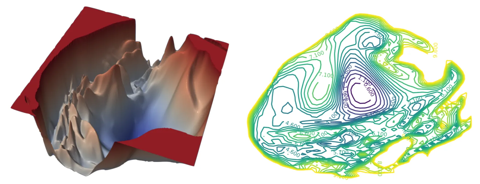
Figure 7.10: This is the loss landscape of ResNet-110-noshort, in both 3D (left) and 2D (right). The paths that SGD takes through these different loss landscapes will be different (Li et al., 2017).

The loss landscape itself remains identical across different training runs—only the starting position changes. Think of this landscape as a fixed mountain range with peaks, valleys, ridges, and basins. This terrain is completely determined by your network architecture (the geological structure), your training data (the climate that shaped it), and your loss function (the elevation measurement system). Every time you train the same architecture on the same data, you're exploring the exact same mountain range. The peaks and valleys never move. What changes is where you start: random initialization is like being blindfolded and dropped at a random location in this mountain range. From each starting point, gradient descent acts like a ball rolling downhill, following the steepest descent toward the nearest valley bottom.

The geometry of these landscapes determines which algorithms are discoverable and robust. Some algorithmic solutions occupy wide, flat valleys where many parameter settings implement similar approaches. Others exist as sharp, narrow peaks that are difficult to find, easy to lose and often misgeneralize under distribution shifts. Algorithms in wide basins remain stable when their parameters are slightly perturbed, corresponding to robust, generalizable solutions (Li et al., 2017). Sharp peaks represent brittle algorithms where tiny changes can cause major performance drops (Keskar et al.; 2017). This geometry matters for goal misgeneralization because the width of different goal-valleys determines their discoverability—wider valleys for misaligned goals make those goals more likely to emerge from training.

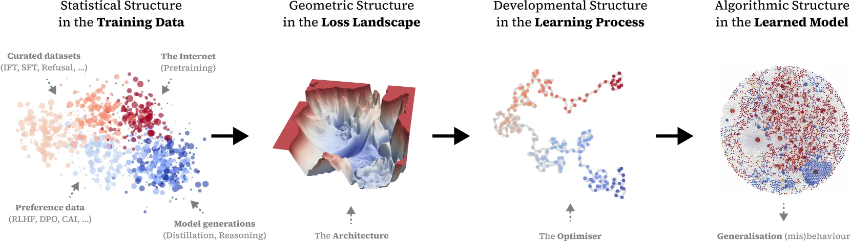
Figure 7.11: From data to model behaviour: Structure in data determines internal structure in models and thus generalisation. Current approaches to alignment work by shaping the training distribution (left), which only indirectly determines model structure (right) through the effects on shaping the optimisation process (middle left & right). To mitigate the limitations of this indirect approach, alignment requires a better understanding of these intermediate links (Lehalleur et al., 2025)

Understanding landscape structure reveals why certain goals systematically emerge over others. The relative size and accessibility of different valleys creates systematic biases in what gets discovered. If the "move right" valley is wider and easier to reach than the "collect coins" valley, training will more often discover the misaligned solution. This landscape structure is determined by the network architecture, training data, and loss function—but most importantly, by the inductive biases that shape which types of algorithms get wide valleys versus narrow peaks.

Definition: Algorithmic Range

The algorithmic range of a machine learning system refers to how extensive the set of algorithms capable of being found is.

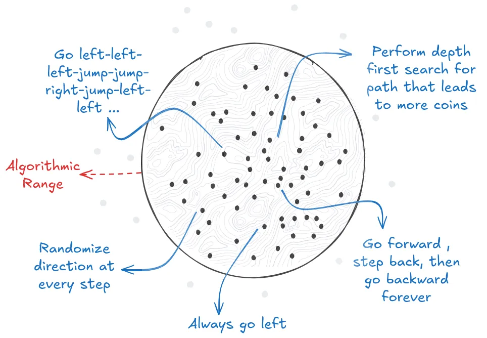
Figure 7.12: A 2D loss landscape where each dot represents a learned algorithm with a different set of parameters on the landscape. There are various different algorithms that the model can learn from the CoinRun example. The goal of SGD is to search through this space for the right dot (set of parameters = learned algorithm).

Path Dependence

Path dependence determines whether different starting points in the loss landscape lead to the same algorithmic destination. In simple landscapes with one dominant valley, almost every starting point rolls into the same solution—that's low path dependence. But complex landscapes contain multiple deep valleys separated by ridges. Now your starting position matters enormously. Drop the ball on the left side of a ridge, and it rolls into Valley A (learning to "move right" in CoinRun). Drop it on the right side, and it rolls into Valley B (learning to "collect coins"). Both valleys represent perfect solutions during training, but they implement completely different algorithms.

Definition: Path Dependence

Path dependence occurs when small differences in the training process lead to discovering fundamentally different algorithms for solving the same task. High path dependence means high variance in learned algorithms across training runs, while low path dependence means consistently finding similar algorithmic solutions.

Path dependence emerges from how gradient descent navigates the loss landscape. Training begins from a random point in parameter space and follows the steepest downhill path toward better performance. When multiple valleys exist—each corresponding to different algorithmic approaches—early random differences can push optimization toward completely different regions. Once committed to descending into a particular valley, gradient descent tends to continue in that direction, making it difficult to escape to other algorithmic solutions.

High path dependence appears when identical training setups discover fundamentally different algorithmic strategies. Researchers trained text classifiers on natural language inference tasks and found that models with identical training performance fell into distinct clusters. Models within each cluster used similar reasoning approaches and could be connected through the loss landscape, but models from different clusters were separated by large performance barriers. One cluster learned bag-of-words approaches while another developed syntactic reasoning strategies (Juneja et al., 2023). Similar variance appears across reinforcement learning experiments and fine-tuning studies where identical setups produce dramatically different learned behaviors.

Low path dependence emerges when mathematical constraints force convergence to the same solution. Delayed generalization, is a phenomenon where a model abruptly transitions from overfitting (performing well only on training data) to generalizing (also called "grokking") (Carvalho et al., 2025). As an example, models learning arithmetic initially memorize training examples and perform poorly on tests. But extended training causes them to suddenly implement the correct mathematical algorithm—consistently the same one across different runs. This suggests that for some tasks, the underlying mathematical structure constrains the solution space so severely that only one good algorithm exists (Mingard et al., 2019). Other evidence includes studies showing gradient descent outcomes correlate with random sampling from parameter distributions.

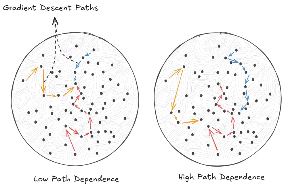
Figure 7.13: A 2D loss landscape where each dot represents a learned algorithm with a different set of parameters on the landscape. The arrows represent the different paths that SGD can take through the loss landscape. If different starting points end up at the same learned algorithm, then we have low path dependence (left), else if different starting points result in different learned algorithms then we have high path dependance (right).

Inductive Bias

Inductive biases describe the shape of the landscape and determine which types of algorithms are more likely to be discovered. If your architecture has a simplicity inductive bias, then this means that algorithmically simple solutions are wide, deep valleys that dominate the loss landscape. Complex solutions might still exist in the landscape, but they're relegated to tiny, hard-to-find peaks. This intuitively explains why the "move right" strategy in CoinRun occupies a massive loss basin spanning huge regions of parameter space, while "navigate to coin-shaped objects" exists only in smaller pockets. You are more likely to find simpler solutions like move right because those basins and valleys are just easier to find and fall into.

Definition: Inductive Bias

Inductive biases are systematic preferences of learning algorithms that favor certain types of solutions over others. These biases emerge from the architecture, optimization procedure, and training setup rather than being explicitly programmed.

Simplicity bias represents the most influential, well studied and potentially dangerous inductive bias for goal misgeneralization. The simplicity bias asks "how complex is it to specify the algorithm in the weights?" This is the ML equivalent of Occam's Razor, which suggests that among competing hypotheses, the one with the fewest assumptions should be selected. SGD seems to subscribe to Occam's Razor, and consistently favors algorithms that rely on simple correlations over complex causal reasoning (Shah et al., 2020; Ren & Sutherland, 2024; Etienne & Flammarion, 2025; Tsoy & Konstantinov, 2024; Carlsmith, 2023)[^note-atlas-1]. In CoinRun, both "move right" and "navigate to coin-shaped objects" could solve the task during training, but "move right" is algorithmically simpler—requiring a single behavioral pattern rather than object recognition, spatial reasoning, and goal-directed navigation. So, the bias exists because simple functions occupy vastly larger volumes in the loss landscape - there are just a lot more ways to encode "move right" than "navigate to coin-shaped objects using visual recognition and spatial reasoning." Empirical work demonstrates that this bias is quite strong, suggesting simple functions are exponentially more likely to emerge than complex ones. (Valle-Pérez et al., 2019). The training process systematically favors the simpler explanation, even when the complex algorithm would generalize better (Valle-Pérez et al., 2019; Shah et al., 2020). This pattern extends broadly to different architectures: image classifiers typically learn texture-based strategies over shape-based ones because texture patterns require simpler computational structures, leading to brittleness when texture and shape provide conflicting signals (Geirhos et al., 2019).

Other inductive biases can create additional systematic preferences that can favor discovering algorithms with misaligned goals. Speed bias looks at "how much computation does the algorithm take at inference time?". An architecture with a speed bias would have wider loss basins with algorithms requiring fewer computational steps, potentially conflicting with solutions that perform more thorough reasoning or long term planning. There are many other examples of biases - frequency bias (learning low-frequency patterns before high-frequency ones) (Rahaman et al., 2019), geometric bias (solutions with lower variability) (Luo et al., 2019), and more. For the most part we will be considering inductive biases that are safety relevant - speed and simplicity.

Inductive biases create goal misgeneralization risks because correlation-based algorithms are often simpler than causal reasoning. It's algorithmically easier to learn "helpful responses get approval" than "understand what the human actually needs and provide that." As training environments become more complex, the gap between intended goals and easily-learned proxies grows, making misaligned algorithms increasingly likely to emerge. The interaction between inductive biases and path dependence determines both the type and specific implementation of learned algorithms—biases constrain training to favor certain solution classes, while path dependence determines which specific implementation within that class gets discovered.

This section on learning dynamics and inductive biases will be especially relevant when we talk about the likelihood of scheming and deceptive alignment.

[^note-atlas-1]: More resources to learn about simplicity bias at this link.

Training is described as rolling into whichever valley is easiest to reach, so simple proxies win by default. Did the loss-landscape account or the empirical examples convince you more? Talk it over with the tutor.